最近在学习MATLAB图像分割部分，现将几个边缘检测算法分享。
有sobel算法、prewitt算法、log算法

图1

图2

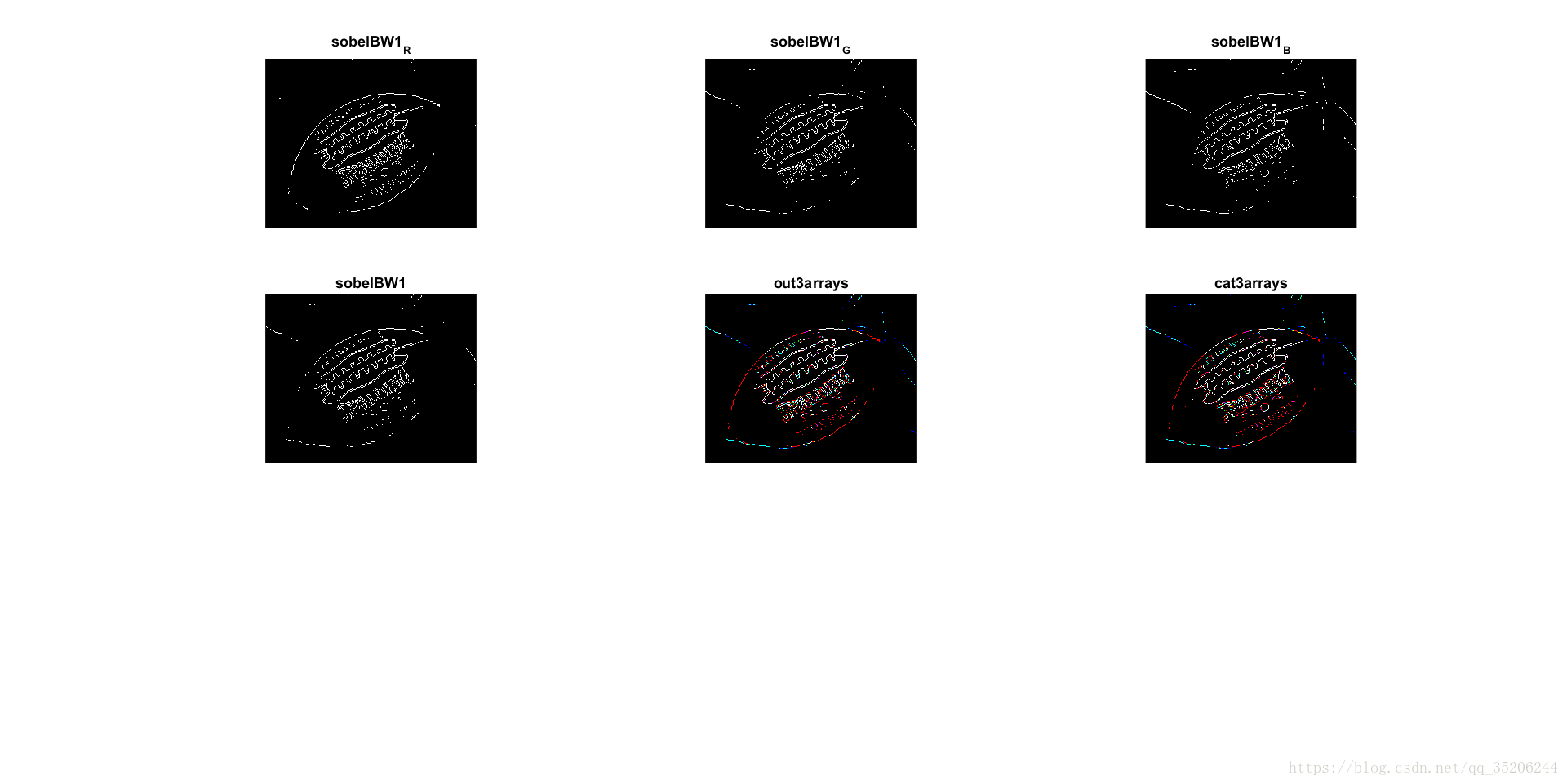
如图2所示，使用sobel算法处理rgb彩色图像
sobelBW1R为彩图R通道提取的边缘，
sobelBW1G为G通道提取的边缘，
sobelBW1B为B通道提取的边缘。
sobelBW1为原图通过rgb2gray处理，直接使用sobel算法提取到的边缘。
out3arrays使用了out方法，将提取的R、G、B通道合成彩色图像输出，
cat3arrays使用了cat方法将提取的R、G、B通道合成彩色图像。

图3
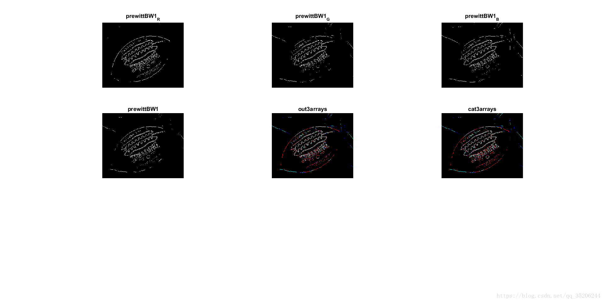
如图3所示，使用prewitt算法处理rbg彩色图像
如图3所示，prewittBW1R为R通道提取的边缘，
prewittBW1G为G通道提取的边缘，
prewittBW1B为B通道提取的边缘，
prewittBW1为原图通过rgb2gray处理，直接使用prewitt算法提取到的边缘，
out3arrays使用了out方法，将提取的R、G、B通道合成彩色图像输出，
cat3arrays使用了cat方法，将提取的R、G、B通道合成彩色图像输出。

图4
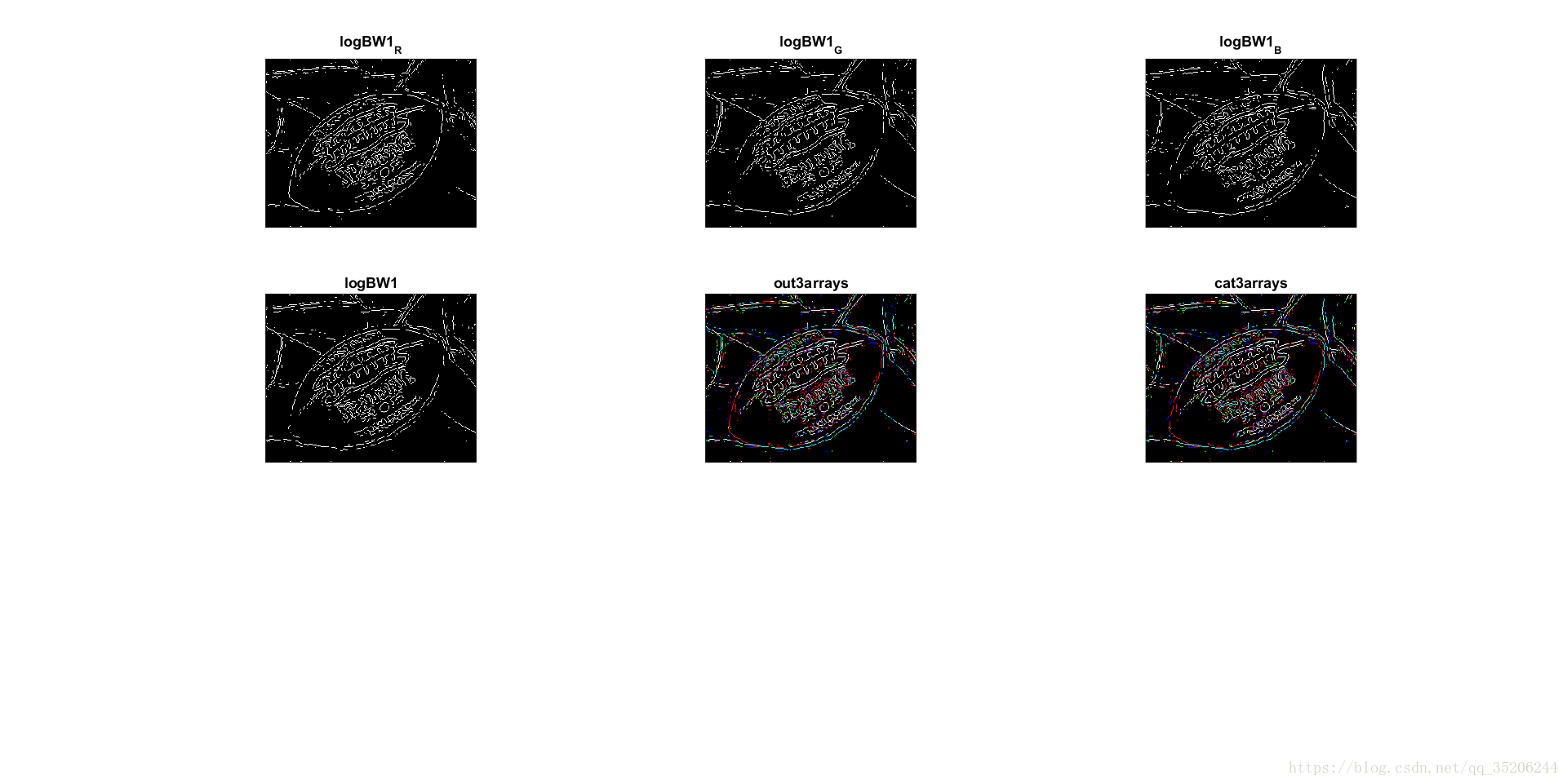
如图3所示，使用log算法处理rbg彩色图像
如图4所示，logBW1R为R通道提取的边缘，
logBW1G为G通道提取的边缘，
logBW1B为B通道提取的边缘。
logBW1为原图通过rgb2gray处理，直接使用log算法提取到的边缘，
out3arrays使用了out方法，将提取的R、G、B通道合成彩色图像输出，
cat3arrays使用了cat方法，将提取到的R、G、B通道合成彩色图像输出。

图5

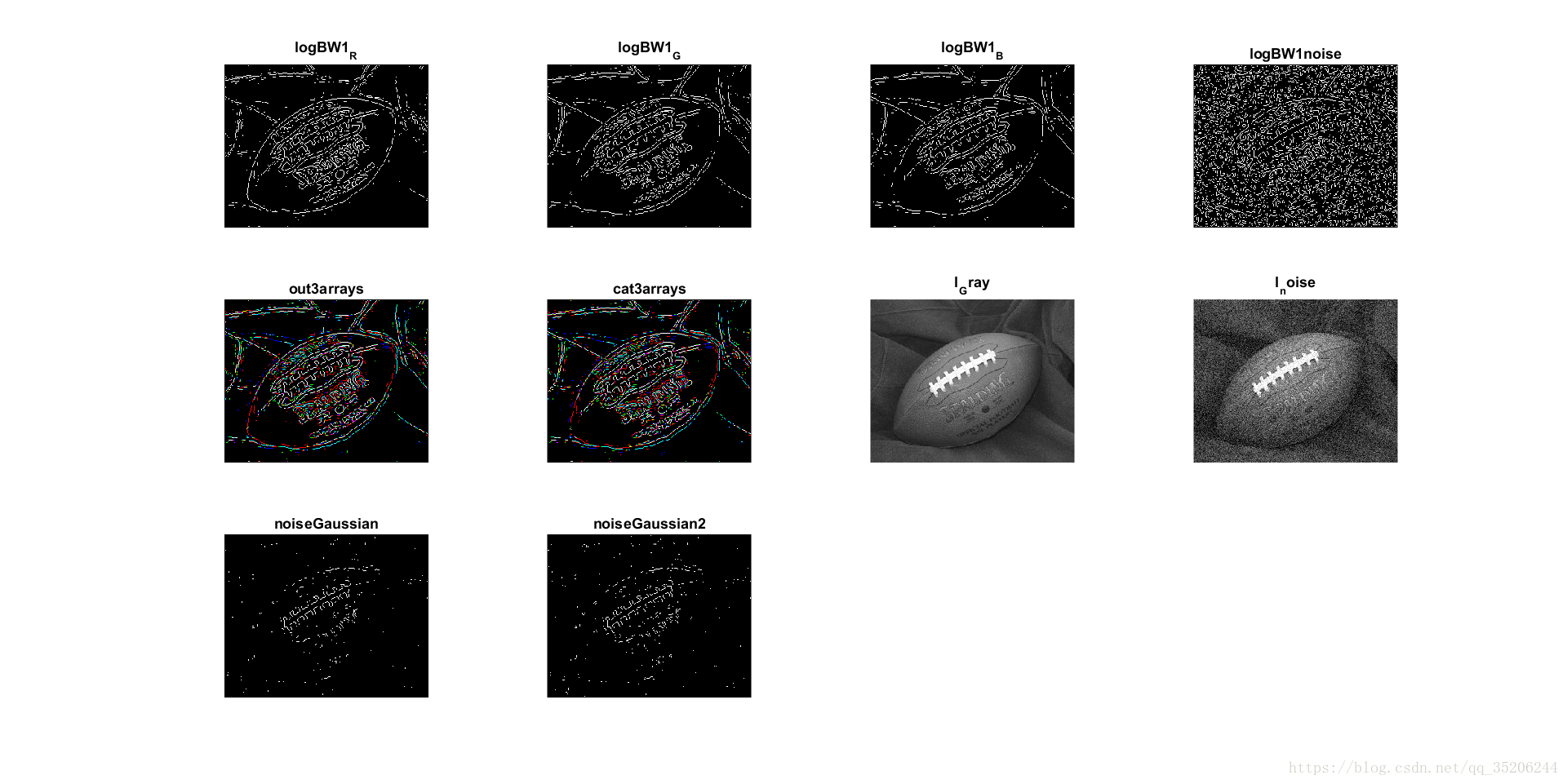
图5在图4所示算法基础上，在原图rgb2gray后，添加了gaussian噪声。

如图5所示，logBW1R为R通道提取的边缘，
logBW1G为G通道提取的边缘，
logBW1B为B通道提取的边缘。
logBW1noise为原图rgb2gray后，添加了gaussian噪声。
logBW1为原图通过rgb2gray处理，直接使用log算法提取到的边缘，
out3arrays使用了out方法，将提取的含有噪声的R、G、B通道合成彩色图像输出，
cat3arrays使用了cat方法，将提取的含有噪声的R、G、B通道合成彩色图像输出。
IGray为原图rgb2gray后的灰度图像，
Inoise为灰度图像添加了gaussian噪声，
noiseGaussian为直接使用log算法处理附加有gaussian噪声的灰度图像，阈值为0.01，
noiseGaussian为直接使用log算法处理附加有gaussian噪声的灰度图像，阈值为0.0095。

sobel算法

I = imread('football.jpg');
I_Gray=rgb2gray(I);
I_R=I(:,:,1);
BW1_R=edge(I_R,'sobel');
figure;
subplot(331);imshow(BW1_R);title('sobelBW1_R');

I_G=I(:,:,2);
BW1_G=edge(I_G,'sobel');
subplot(332);imshow(BW1_G);title('sobelBW1_G');

I_B=I(:,:,3);
BW1_B=edge(I_B,'sobel');
subplot(333);imshow(BW1_B);title('sobelBW1_B');

BW1=edge(I_Gray,'sobel');
subplot(334);imshow(BW1);title('sobelBW1');


out(:,:,1)=BW1_R;
out(:,:,2)=BW1_G;
out(:,:,3)=BW1_B;
subplot(335);imshow(double(out),[]);title('out3arrays');
out2=cat(3,BW1_R,BW1_G,BW1_B);
subplot(336);imshow(double(out2),[]);title('cat3arrays');

prewitt算法

I = imread('football.jpg');
I_Gray=rgb2gray(I);
I_R=I(:,:,1);
BW1_R=edge(I_R,'prewitt');
figure;
subplot(331);imshow(BW1_R);title('prewittBW1_R');

I_G=I(:,:,2);
BW1_G=edge(I_G,'prewitt');
subplot(332);imshow(BW1_G);title('prewittBW1_G');

I_B=I(:,:,3);
BW1_B=edge(I_B,'prewitt');
subplot(333);imshow(BW1_B);title('prewittBW1_B');

BW1=edge(I_Gray,'prewitt');
subplot(334);imshow(BW1);title('prewittBW1');


out(:,:,1)=BW1_R;
out(:,:,2)=BW1_G;
out(:,:,3)=BW1_B;
subplot(335);imshow(double(out),[]);ylabel('out3arrays');
out2=cat(3,BW1_R,BW1_G,BW1_B);
subplot(336);imshow(double(out2),[]);xlabel('cat3arrays');

log算法

I = imread('football.jpg');
I_Gray=rgb2gray(I);
I_noise=imnoise(I_Gray,'gaussian');

I_R=I(:,:,1);
BW1_R=edge(I_R,'log');
figure;
subplot(341);imshow(BW1_R);title('logBW1_R');

I_G=I(:,:,2);
BW1_G=edge(I_G,'log');
subplot(342);imshow(BW1_G);title('logBW1_G');

I_B=I(:,:,3);
BW1_B=edge(I_B,'log');
subplot(343);imshow(BW1_B);title('logBW1_B');

BW1=edge(I_noise,'log');
subplot(344);imshow(BW1);title('logBW1noise');


out(:,:,1)=BW1_R;
out(:,:,2)=BW1_G;
out(:,:,3)=BW1_B;
subplot(345);imshow(double(out),[]);title('out3arrays');
out2=cat(3,BW1_R,BW1_G,BW1_B);
subplot(346);imshow(double(out2),[]);title('cat3arrays');
subplot(347);imshow(I_Gray);title('I_Gray');

subplot(348);imshow(I_noise);title('I_noise');
BW1_noiseGaussian=edge(I_noise,'log',0.01);
subplot(349);imshow(BW1_noiseGaussian);title('noiseGaussian');
BW1_noiseGaussian2=edge(I_noise,'log',0.0095);
subplot(3,4,10);imshow(BW1_noiseGaussian2);title('noiseGaussian2');

总结：
通过3种算法的对比，可见，sobel和prewitt在检测边缘方面，效果很相近，log在检测边缘方面，可以检测出更细节的部分，且log可处理部分噪声（以gaussian噪声为例）。

时间仓促，笔者能力有限，如有错误，欢迎指出。