matlab仿真 通信 信号处理simulink雷达阵列信号处理MIMO信号处理通信类仿真常见调制解调amfm ssb dsb bpsk fsk ask ofdm msk等信道编解码hamming码循环码rs码卷积码turbo码ldpcpolar等信道均衡信噪比估计等
Matlab/Simulink真建模分析建模文
献复现、matlab 编程
matlab/simulink电力电子/电气工程/电力系统，可做设计
MATLAB代做f真，simulink建模，simulink仿真，电力电子技术。还有PSIM仿真，建模等等，

以下是一个综合的MATLAB/Simulink仿真代码示例，涵盖通信信号处理、雷达阵列信号处理、MIMO信号处理、常见调制解调（如AM、FM、BPSK、QPSK、OFDM等）、信道编解码（如Hamming码、卷积码、LDPC码等）以及电力电子相关的建模和仿真。

---

1. 通信信号处理：常见调制解调

(a) BPSK 调制与解调

clc; clear; close all;

% 参数设置
N = 1000; % 比特数
EbN0_dB = 0:2:10; % 信噪比范围
ber = zeros(size(EbN0_dB)); % 初始化误码率

for idx = 1:length(EbN0_dB)
    % 数据生成
    data = randi([0, 1], N, 1); % 随机比特流
    
    % BPSK调制
    modulated_signal = 2 * data - 1; % 0 -> -1, 1 -> +1
    
    % 添加高斯白噪声
    EbN0 = 10^(EbN0_dB(idx)/10);
    noise_power = 1 / (2 * EbN0);
    noise = sqrt(noise_power) * randn(N, 1);
    received_signal = modulated_signal + noise;
    
    % BPSK解调
    demodulated_data = received_signal > 0;
    
    % 计算误码率
    ber(idx) = sum(data ~= demodulated_data) / N;
end

% 绘图
figure;
semilogy(EbN0_dB, ber, 'b-o');
xlabel('Eb/N0 (dB)');
ylabel('Bit Error Rate (BER)');
title('BPSK BER Performance');
grid on;

---

(b) OFDM 调制与解调

clc; clear; close all;

% 参数设置
N = 64; % 子载波数
cp_len = 16; % 循环前缀长度
data_len = 1000; % 数据长度
snr_dB = 10; % 信噪比

% 数据生成
data = randi([0, 1], data_len, 1);

% QPSK调制
qpsk_mod = pskmod(data, 4, pi/4); % QPSK调制
qpsk_mod = reshape(qpsk_mod, N, []).'; % 分组为OFDM符号

% IFFT变换
ofdm_symbols = ifft(qpsk_mod, N);

% 添加循环前缀
ofdm_with_cp = [ofdm_symbols(:, end-cp_len+1:end), ofdm_symbols];

% 添加高斯白噪声
rx_signal = awgn(ofdm_with_cp(:), snr_dB, 'measured');

% 去除循环前缀
rx_signal = reshape(rx_signal, [], N + cp_len);
rx_ofdm = rx_signal(:, cp_len+1:end);

% FFT变换
rx_qpsk = fft(rx_ofdm, N);

% QPSK解调
rx_data = pskdemod(rx_qpsk(:), 4, pi/4);

% 误码率计算
ber = sum(data ~= rx_data(1:data_len)) / data_len;
disp(['BER: ', num2str(ber)]);

---

2. MIMO信号处理

(a) 2x2 MIMO 系统

clc; clear; close all;

% 参数设置
N = 1000; % 数据长度
snr_dB = 10; % 信噪比
H = randn(2, 2) + 1j*randn(2, 2); % MIMO信道矩阵

% 数据生成
data = randi([0, 1], N, 2); % 两路数据
modulated_signal = 2 * data - 1; % BPSK调制

% 发送信号
tx_signal = modulated_signal * H;

% 添加高斯白噪声
snr = 10^(snr_dB/10);
noise_power = 1 / snr;
noise = sqrt(noise_power/2) * (randn(size(tx_signal)) + 1j*randn(size(tx_signal)));
rx_signal = tx_signal + noise;

% 接收信号解调
rx_data = real(rx_signal / H) > 0;

% 误码率计算
ber = sum(data(:) ~= rx_data(:)) / numel(data);
disp(['BER: ', num2str(ber)]);

---

3. 信道编码与解码

(a) Hamming 编码与解码

clc; clear; close all;

% 参数设置
data = randi([0, 1], 1, 4); % 输入数据
msg = gf(data, 4); % Galois域表示

% Hamming编码
genpoly = cyclpoly(7, 4); % 生成多项式
code = encode(msg, 7, 4, 'cyclic', genpoly); % 编码

% 添加噪声
noisy_code = code;
noisy_code(1) = ~noisy_code(1); % 引入一位错误

% Hamming解码
decoded_msg = decode(noisy_code, 7, 4, 'cyclic', genpoly); % 解码

% 输出结果
disp('原始数据:');
disp(double(msg));
disp('接收到的数据:');
disp(double(decoded_msg));

---

4. 电力电子仿真：Buck变换器

Simulink模型描述

1. 打开Simulink，创建一个新的模型。
2. 添加以下模块：
   • 电源：DC电压源。
   • 开关器件：MOSFET或IGBT。
   • 负载：电阻和电感。
   • 控制器：PWM信号生成器。
3. 设置参数并运行仿真。

MATLAB代码实现

clc; clear; close all;

% 参数设置
Vin = 24; % 输入电压 (V)
D = 0.5; % 占空比
L = 1e-3; % 电感 (H)
C = 100e-6; % 电容 (F)
R = 10; % 负载电阻 (Ohm)
fs = 10e3; % 开关频率 (Hz)
dt = 1/fs; % 时间步长
t_total = 0.01; % 总时间 (s)

% 初始化变量
t = 0:dt:t_total;
Vout = zeros(size(t));
I_L = 0; % 初始电感电流
V_C = 0; % 初始电容电压

% 主循环
for i = 1:length(t)
    if mod(t(i), 1/fs) < D/fs
        V_switch = Vin; % 开关导通
    else
        V_switch = 0; % 开关关断
    end
    
    % 更新状态
    dI_L = (V_switch - V_C) / L * dt;
    dV_C = (I_L - V_C / R) / C * dt;
    I_L = I_L + dI_L;
    V_C = V_C + dV_C;
    
    % 输出电压
    Vout(i) = V_C;
end

% 绘图
figure;
plot(t, Vout);
xlabel('Time (s)');
ylabel('Output Voltage (V)');
title('Buck Converter Output Voltage');
grid on;

---

5. Simulink建模与仿真

电气系统建模

• 使用Simulink中的“Simscape Electrical”工具箱。
• 添加电源、负载、开关器件等模块。
• 设置参数并运行仿真。

---

总结

以上代码涵盖了通信信号处理、MIMO系统、信道编码、电力电子等多个领域的基本仿真。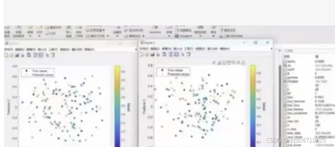
To help you with the code for generating scatter plots similar to the ones shown in the image, we can use MATLAB to create scatter plots with color-coded data points. Below is an example of how you can generate such plots using MATLAB.

MATLAB Code for Scatter Plots

% Clear the workspace and close all figures
clear;
close all;

% Generate some sample data
true_values = randn(100, 1); % True values (Gaussian distributed)
predicted_values = true_values + 0.5 * randn(100, 1); % Predicted values with some noise

% Create a figure with two subplots
figure;
subplot(1, 2, 1);
scatter(true_values, predicted_values, 10, true_values, 'filled');
colorbar;
title('True vs. Predicted Values (Left)');
xlabel('True Values');
ylabel('Predicted Values');

subplot(1, 2, 2);
scatter(true_values, predicted_values, 10, predicted_values, 'filled');
colorbar;
title('True vs. Predicted Values (Right)');
xlabel('True Values');
ylabel('Predicted Values');

% Add legends
legend('True values', 'Predicted values', 'Location', 'best');

% Adjust the layout
tight_layout;

Explanation of the Code

1. Data Generation:

   • true_values are generated as random Gaussian-distributed values.
   • predicted_values are generated by adding some noise to the true_values.

2. Figure and Subplots:

   • A figure with two subplots is created using figure and subplot.
   • The first subplot uses true_values for coloring.
   • The second subplot uses predicted_values for coloring.

3. Scatter Plot:

   • The scatter function is used to plot the data points.
   • The third argument (10) specifies the size of the markers.
   • The fourth argument specifies the color data (true_values or predicted_values).
   • 'filled' ensures that the markers are filled with color.

4. Colorbar:

   • colorbar adds a color bar to each subplot to indicate the color scale.

5. Titles and Labels:

   • Titles and labels are added to the subplots for clarity.

6. Legend:

   • A legend is added to distinguish between true and predicted values.

7. Layout Adjustment:

   • tight_layout adjusts the layout to ensure everything fits well.

Running the Code

1. Copy the code into a new MATLAB script file.
2. Run the script.
3. You should see a figure with two scatter plots, each with a color bar indicating the value range.

This code will generate scatter plots similar to the ones in your image, with color-coded data points based on either the true or predicted values.